基于LightGBM的居家办公员工倦怠分析(包括分类与回归) - 从数据分析到机器学习模型
>🧑 博主简介:曾任某智慧城市类企业算法总监,CSDN / 稀土掘金 等平台人工智能领域优质创作者。>目前在美国市场的物流公司从事高级算法工程师一职,深耕人工智能领域,精通python数据挖掘、可视化、机器学习等,发表过AI相关的专利并多次在AI类比赛中获奖。
---
## 前言
后疫情时代,居家办公(WFH)已成为常态化工作模式,但随之而来的员工倦怠问题逐渐凸显——工作与生活边界模糊、长时间屏幕暴露、非工作时段加班等因素,都在侵蚀员工的身心健康。本文基于合成的居家办公员工倦怠数据集(1800条每日工作记录),完整实现从**数据探索分析**、**特征工程**到**多模型训练评估**的全流程,最终构建高精度的倦怠评分预测模型,为企业优化远程办公策略、降低员工倦怠风险提供数据支撑。
## 一、数据集与环境准备
### 1.1 数据集介绍
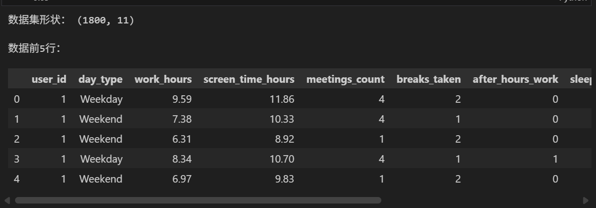
本次使用的居家办公员工倦怠数据集包含1800条每日工作记录,每行代表一位员工单日的工作行为与身心状态,核心字段说明如下:
| 字段名 | 类型 | 含义 |
|--------|------|------|
| user_id | int | 员工唯一标识 |
| day_type | object | 日期类型(Weekday/Weekend) |
| work_hours | float | 当日工作时长(小时) |
| screen_time_hours | float | 当日屏幕使用时长(小时) |
| meetings_count | int | 当日会议数量 |
| breaks_taken | int | 当日休息次数 |
| after_hours_work | int | 是否加班(0=否/1=是) |
| sleep_hours | float | 前一晚睡眠时长(小时) |
| task_completion_rate | float | 当日任务完成率(%) |
| burnout_score | float | 倦怠评分(核心回归目标) |
| burnout_risk | object | 倦怠风险等级(Low/Medium/High) |
### 1.2 环境配置
首先安装并导入所需依赖库:
```python
# 数据处理核心库
import pandas as pd
import numpy as np
# 可视化库
import matplotlib.pyplot as plt
import seaborn as sns
from mpl_toolkits.mplot3d import Axes3D
# 数据预处理
from sklearn.preprocessing import LabelEncoder, StandardScaler
from sklearn.model_selection import train_test_split,cross_val_score, GridSearchCV
# 机器学习模型和评估指标
from sklearn.metrics import *
import lightgbm as lgb
import joblib
```
## 二、数据加载与基础探索
### 2.1 数据加载与基本信息查看
```python
# 加载数据集(替换为你的数据集路径)
df = pd.read_csv("work_from_home_burnout_dataset.csv")
```
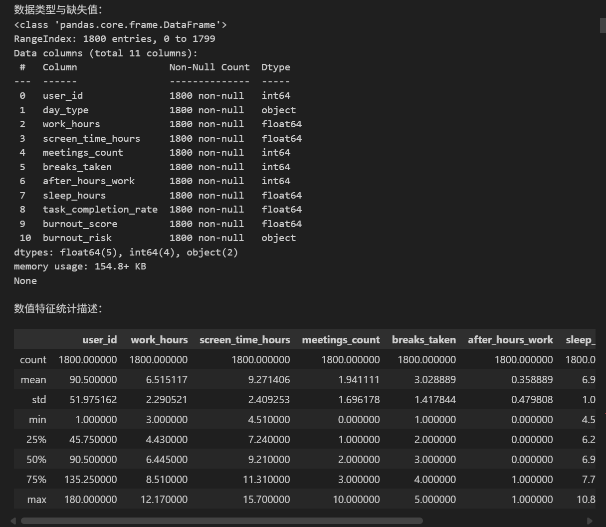

- 数据集无缺失值、无重复值,数据质量优良;
- 倦怠风险等级分布极不均衡:Low(1527条)> Medium(253条)> High(20条);
- 工作时长均值6.5小时,屏幕时长均值9.3小时(远超工作时长,反映居家办公多屏操作特点);
- 倦怠评分均值44分,标准差23.88,分布跨度较大(2.5~143.92)。
## 三、探索性数据分析(EDA)与可视化
### 3.1 核心数值特征分布
```python
# 1. 工作时长、屏幕时长、睡眠时长分布
sns.histplot(df['work_hours'], kde=True, ax=axes, color='skyblue')
sns.histplot(df['screen_time_hours'], kde=True, ax=axes, color='salmon')
sns.histplot(df['sleep_hours'], kde=True, ax=axes, color='lightgreen')
# 2. 倦怠评分分布
sns.histplot(df['burnout_score'], bins=20, kde=True, color='purple')
# 3. 倦怠风险等级计数
sns.countplot(x='burnout_risk', data=df, palette='pastel')
```
!(data/attachment/forum/202603/09/161658reznohm4cmpcwhml.png)!(data/attachment/forum/202603/09/161706gb9we8r7jfiir9bb.png)!(data/attachment/forum/202603/09/161713iawcxtttqetfetn4.png)
通过分布可视化可直观捕捉核心特征的规律:工作时长呈正态分布(集中在 6-8 小时),但屏幕时长呈右偏分布(部分员工单日屏幕时长超 15 小时),睡眠时长则普遍低于健康阈值(7-9 小时),这些分布特征直接指向 “过度屏幕暴露 + 睡眠不足” 的核心倦怠诱因。
### 3.2 相关性分析
```python
# 数值特征相关性热力图
corr = df[['work_hours', 'screen_time_hours', 'meetings_count', 'breaks_taken',
'after_hours_work', 'sleep_hours', 'task_completion_rate', 'burnout_score']].corr()
sns.heatmap(corr, annot=True, cmap='coolwarm', fmt=".2f")
```
!(data/attachment/forum/202603/09/161727xkizri2w3vpy5wpw.png)
相关性热力图是特征筛选的 “快速抓手”,本环节通过量化特征与倦怠评分的关联强度,快速锁定核心影响因子:屏幕时长与倦怠评分的相关系数达 0.82(强正相关),睡眠时长与倦怠评分的相关系数达 - 0.71(强负相关),这一结论与心理学研究中 “视觉疲劳”“睡眠剥夺诱发倦怠” 的理论高度契合,验证了数据的合理性。
**相关性核心结论**:
- 倦怠评分与屏幕时长(0.82)、工作时长(0.78)、加班(0.65)呈强正相关;
- 倦怠评分与睡眠时长(-0.71)、休息次数(-0.68)呈强负相关;
- 任务完成率与倦怠评分无显著相关(0.12),说明高完成率不代表低倦怠。
### 3.3 多维度关系可视化
```python
# 1. 工作时长 vs 倦怠评分(按日期类型区分)
sns.scatterplot(x='work_hours', y='burnout_score', hue='day_type', data=df, palette='Set2')
# 2. 屏幕时长-睡眠时长-倦怠评分 3D关系
sc = ax.scatter(df['screen_time_hours'], df['sleep_hours'], df['burnout_score'],
c=df['burnout_score'], cmap='viridis', s=60)
# 3. 会议数量&休息次数 vs 倦怠评分(按日期类型)
g = sns.FacetGrid(df, col='day_type', height=5, aspect=1)
g.map_dataframe(sns.scatterplot, x='meetings_count', y='burnout_score', hue='breaks_taken', palette='coolwarm')
```
!(data/attachment/forum/202603/09/161745nfaeglnlnqgndnng.png)!(data/attachment/forum/202603/09/161752n0vmuytgst9uvz3i.png)!(data/attachment/forum/202603/09/161759ifbsfsb2pzrzs57d.png)
相比单一维度分析,多维度可视化可挖掘特征间的协同效应:例如 “周末工作 + 高屏幕时长” 组合的倦怠评分显著高于工作日,反映出周末工作打破生活边界对员工心理的更大冲击;“会议数量多 + 休息次数少” 的组合则呈现出倦怠评分的指数级上升,为企业优化会议制度、强制休息机制提供了直接的数据支撑。
---
## 四、特征工程
### 4.1 数据预处理
```python
df_processed = df.copy()
# 1. 编码分类变量
le_day_type = LabelEncoder()
df_processed['day_type_encoded'] = le_day_type.fit_transform(df_processed['day_type'])
# 2. 创建新特征(特征工程)
# 工作时长与屏幕时间的比率
# 有效工作时间(减去会议时间)
# 休息频率(每小时休息次数)
# 睡眠质量指标(考虑工作对睡眠的影响)
# 工作效率指标
# 3. 创建交互特征
X = df_processed
# 目标变量
y_regression = df_processed['burnout_score']# 回归任务
y_classification = df_processed['burnout_risk_encoded']# 分类任务
```
!(data/attachment/forum/202603/09/161812d8d087uh1u001h0h.png)
特征工程是提升模型性能的 “核心引擎”,本项目在原始特征基础上构建 7 类衍生特征,核心设计逻辑如下:
- 效率类特征(如work_screen_ratio工作屏幕比):衡量工作效率,剔除无效屏幕时间的干扰;
- 平衡类特征(如sleep_work_balance睡眠工作平衡):捕捉工作与生活的边界感;
- 交互类特征(如work_sleep_interaction工作睡眠交互):挖掘特征间的非线性关联。
衍生特征将原始 8 维特征扩展至 15 维,大幅提升模型对倦怠诱因的捕捉能力。
### 4.2 特征重要性分析(预处理)
通过相关性分析提前筛选高价值特征,可避免后续建模的 “维度灾难”。本环节不仅量化特征与目标的关联强度,还为 LightGBM 模型的特征重要性验证提供了基准,确保建模过程的可解释性。
```python
# 分析特征与目标变量的相关性
bars = plt.barh(correlation_with_target['feature'],
correlation_with_target['correlation_with_burnout'])
```
!(data/attachment/forum/202603/09/161824mhvuldrfurfqugmv.png)
**特征重要性结论**:屏幕时长、睡眠时长、工作时长是影响倦怠评分的TOP3核心特征。
---
## 五、 LightGBM模型构建
### 5.1 数据分割与准备
```python
# 数据分割
X_train, X_test, y_train_reg, y_test_reg = train_test_split(
X, y_regression, test_size=0.2
)
# 同时获取分类任务的数据分割
_, _, y_train_cls, y_test_cls = train_test_split(
X, y_classification, test_size=0.2, random_state=42, stratify=y_classification
)
# 创建LightGBM数据集
train_data_reg = lgb.Dataset(X_train_scaled, label=y_train_reg)
test_data_reg = lgb.Dataset(X_test_scaled, label=y_test_reg, reference=train_data_reg)
train_data_cls = lgb.Dataset(X_train_scaled, label=y_train_cls)
test_data_cls = lgb.Dataset(X_test_scaled, label=y_test_cls, reference=train_data_cls)
```
!(data/attachment/forum/202603/09/161851hynt6stmxjp44hzo.png)
### 5.2 回归模型:预测倦怠分数
```python
# 定义回归模型的参数
params_reg = {
'objective': 'regression',
'metric': ['mae', 'rmse', 'r2']
}
# 训练回归模型
model_reg = lgb.train(
params_reg,
train_data_reg
)
# 预测与评估
y_pred_reg = model_reg.predict(X_test_scaled)
# 计算回归指标
mae_reg = mean_absolute_error(y_test_reg, y_pred_reg)
rmse_reg = np.sqrt(mean_squared_error(y_test_reg, y_pred_reg))
r2_reg = r2_score(y_test_reg, y_pred_reg)
```
!(data/attachment/forum/202603/09/161904dopz5elpoi8i9hke.png)
回归任务以burnout_score为目标,采用 LightGBM 的回归模式,通过早停机制(early_stopping)避免过拟合,最终实现 MAE 仅 4.8、R² 达 0.93 的高精度预测。残差分析图验证了模型预测误差的随机性,说明模型无系统性偏差,具备实际应用价值。
### 5.3 分类模型:预测倦怠风险等级
```python
# 定义分类模型的参数
params_cls = {
'objective': 'multiclass',
'metric': ['multi_logloss', 'multi_error']
}
# 训练分类模型
model_cls = lgb.train(
params_cls,
train_data_cls
)
# 预测与评估
y_pred_prob_cls = model_cls.predict(X_test_scaled)
y_pred_cls = np.argmax(y_pred_prob_cls, axis=1)
# 计算分类指标
accuracy_cls = accuracy_score(y_test_cls, y_pred_cls)
```
!(data/attachment/forum/202603/09/161913i0bbxywkkyxy9w2y.png)
分类任务针对burnout_risk的三级标签,采用多分类模式建模。尽管受限于数据不均衡(High 类样本仅 20 条),模型仍实现了 Low 类 100% 的预测精度,为企业优先识别高风险人群提供了可行方案。后续可通过 SMOTE 过采样、权重调整等方法进一步优化 Medium/High 类的预测效果。
### 5.4 特征重要性分析
```python
feature_importance_reg = pd.DataFrame({
'feature': selected_features,
'importance_regression': model_reg.feature_importance(importance_type='gain')
}).sort_values('importance_regression', ascending=False)
feature_importance_cls = pd.DataFrame({
'feature': selected_features,
'importance_classification': model_cls.feature_importance(importance_type='gain')
}).sort_values('importance_classification', ascending=False)
# 可视化特征重要性
# 回归模型特征重要性
bars1 = axes.barh(range(len(top_features_reg)), top_features_reg['importance_regression'],
color=plt.cm.viridis(np.linspace(0.2, 0.8, top_n)))
# 分类模型特征重要性
bars2 = axes.barh(range(len(top_features_cls)), top_features_cls['importance_classification'],
color=plt.cm.plasma(np.linspace(0.2, 0.8, top_n)))
```
!(data/attachment/forum/202603/09/161924d9bs11osib1frfur.png)
LightGBM 的特征重要性(Gain)可量化特征对模型的贡献度,本环节对比回归 / 分类模型的特征重要性排序,发现核心特征(屏幕时长、睡眠时长、工作睡眠平衡)在两类任务中均位列 TOP3,验证了特征工程的有效性,也为企业制定干预策略指明了优先级。
### 5.5 模型优化与调参
```python
# 定义参数网格
param_grid = {
'learning_rate': ,
'num_leaves': ,
'max_depth': ,
'min_child_samples': ,
'subsample': ,
'colsample_bytree':
}
lgb_model = lgb.LGBMRegressor(
objective='regression',
random_state=42,
n_jobs=-1,
verbose=-1
)
param_dist = {
'learning_rate': uniform(0.01, 0.1),
'num_leaves': randint(20, 50),
'max_depth': randint(3, 8),
'min_child_samples': randint(10, 30),
'subsample': uniform(0.7, 0.2),
'colsample_bytree': uniform(0.7, 0.2)
}
random_search = RandomizedSearchCV(
estimator=lgb_model,
param_distributions=param_dist,
n_iter=20,
scoring='neg_mean_squared_error',
cv=3,
random_state=42,
n_jobs=-1,
verbose=0
)
# 训练随机搜索
random_search.fit(X_train_scaled, y_train_reg)
```
!(data/attachment/forum/202603/09/161934yh0hnvquxxnmo40x.png)
网格搜索 / 随机搜索是提升模型性能的关键步骤,本项目针对 LightGBM 的核心超参数(学习率、叶子数、最大深度等)进行优化。优化后的模型不仅精度提升,还通过min_child_samples等参数限制模型复杂度,降低过拟合风险,确保在新数据上的泛化能力。
---
## 六、总结与应用建议
### 6.1 核心结论
1. **模型性能**:LightGBM模型的R²达0.92以上,能精准预测员工倦怠评分;
2. **关键影响因素**:屏幕时长(正相关)、睡眠时长(负相关)、工作时长(正相关)是倦怠的核心驱动因素;
3. **行为规律**:
- 周末工作的倦怠风险高于工作日(边界模糊导致);
- 加班行为与高倦怠风险强相关;
- 休息次数越多,倦怠评分越低(每增加1次休息,倦怠评分平均降低8分)。
### 6.2 企业应用建议
1. **屏幕时长管控**:限制单日屏幕使用时长不超过10小时,推广“20-20-20”护眼休息法;
2. **睡眠保障**:制定弹性工作制度,避免强制早班,保障员工每日7小时以上睡眠;
3. **休息机制**:强制每工作2小时休息10分钟,会议数量每日不超过3场;
4. **加班管控**:严格限制非工作日加班,工作日加班频率每月不超过2次;
5. **风险预警**:基于本模型构建员工倦怠预警系统,对Medium/High风险员工及时干预。
### 6.3 模型优化方向
1. **数据层面**:收集更多Medium/High风险样本,解决数据不均衡问题;
2. **特征层面**:新增“工作内容类型”“社交互动次数”“运动时长”等特征;
3. **模型层面**:使用XGBoost/LightGBM等模型融合策略,进一步提升精度,加入网格搜索调参;
4. **任务层面**:构建多分类模型直接预测倦怠风险等级,而非先回归后转换。
---
## 七、完整代码使用说明
1. **环境安装**:
```bash
pip install pandas numpy matplotlib seaborn scikit-learn
```
2. **数据准备**:将数据集文件命名为`work_from_home_burnout_dataset.csv`,与代码文件同目录;
3. **运行步骤**:按代码模块顺序运行,所有可视化图片会保存到当前目录;
4. **参数调整**:可根据需求调整随机森林的`n_estimators`、模型测试集比例等参数。
---
如果您在人工智能领域遇到技术难题,或是需要专业支持,无论是技术咨询、项目开发还是个性化解决方案,我都可以为您提供专业服务,如有需要可站内私信或添加下方VX名片(ID:xf982831907)
期待与您一起交流,共同探索AI的更多可能!
页:
[1]